Metacognitive efficiency with meta-d′

Level Intermediate · Time 20 minutes · Prerequisites basic signal detection theory · cpm components EstimatorMetaD · Data load_metacognition_data

Metacognition is the ability to monitor and evaluate our own decisions. One way to measure it is to ask people how confident they are after each decision: if their metacognition is good, they are more confident when they are right than when they are wrong.

Meta-d′ (Maniscalco & Lau, 2012) measures how well confidence ratings discriminate correct from incorrect decisions, in the same units as the sensitivity of the decisions themselves, \(d'\). In this example, we estimate meta-d′ with EstimatorMetaD for participants of a perceptual decision-making task.

What you’ll learn

• what \(d'\), meta-\(d'\) and the M-ratio measure,

• how to prepare trial-level decision and confidence data,

• how to estimate meta-\(d'\) for each participant, and interpret the estimates.

import cpm
import numpy as np
import pandas as pd
import matplotlib.pyplot as plt

print(cpm.__version__)
np.random.seed(2026)

0.25.7.dev0

Meta-d′ in brief

In signal detection theory, \(d'\) measures how well an observer discriminates two stimulus classes, S1 and S2, from the distance between the internal evidence distributions of the two classes. This is the type 1 task: deciding which stimulus was shown.

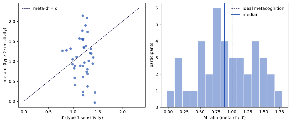
The type 2 task is to discriminate one’s own correct decisions from incorrect ones with confidence ratings. Meta-\(d'\) is the \(d'\) that an ideal metacognitive observer would need to produce the confidence ratings we observe. If confidence uses all the information that the decision was based on, meta-\(d'\) equals \(d'\). If information is lost between the decision and the confidence rating, meta-\(d'\) is smaller than \(d'\).

Because meta-\(d'\) and \(d'\) are in the same units, their ratio, the M-ratio, is a measure of metacognitive efficiency that does not depend on how good the decisions themselves are (Fleming & Lau, 2014):

\[ \text{M-ratio} = \frac{\text{meta-}d'}{d'} \]

An M-ratio of 1 means ideal metacognition; values below 1 mean that confidence is less informative than it could be.

The data

The data come from a perceptual decision-making task with confidence ratings, played on smartphones as part of the BrainExplorer platform (Marzuki et al., 2025). On each trial, participants saw a brief display of two kinds of aliens and decided which kind was more numerous, then rated their confidence from 0 (“totally guessing”) to 100 (“totally certain”).

from cpm.datasets import load_metacognition_data

data = load_metacognition_data()
data.head()

	participant	signal	stimulus_intensity	response	confidence	accuracy
0	1	1	8	0	56	0
1	1	0	12	0	65	1
2	1	0	12	1	22	0
3	1	1	16	1	62	1
4	1	0	16	0	60	1

The columns are:

• participant: the participant number,

• signal: which kind of alien was more numerous (0 for S1, 1 for S2),

• stimulus_intensity: the difference in the number of aliens, which a staircase adjusted to keep accuracy at about 70%,

• response: the decision of the participant (0 for S1, 1 for S2),

• confidence: the confidence rating (0 to 100),

• accuracy: whether the decision was correct.

trials = data.groupby("participant").size()
print(f"{data.participant.nunique()} participants, {trials.median():.0f} trials each, accuracy {data.accuracy.mean():.2f}")

300 participants, 80 trials each, accuracy 0.73

Before fitting anything, we can check whether confidence tracks accuracy at all: on average, participants should be more confident when they are correct.

confidence = data.groupby(["participant", "accuracy"]).confidence.mean().unstack()

fig, ax = plt.subplots(figsize=(5, 4.5))
ax.scatter(confidence[0], confidence[1], alpha=0.5, color="#2350b0", edgecolor="none")
ax.plot([0, 100], [0, 100], color="#0c0c45", linestyle="--", linewidth=1)
ax.set_xlabel("mean confidence, incorrect trials")
ax.set_ylabel("mean confidence, correct trials")
ax.set_xlim(0, 100)
ax.set_ylim(0, 100)
plt.tight_layout()
plt.show()

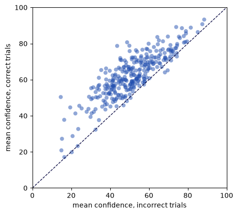
Most participants lie above the diagonal: they are more confident when they are correct. Meta-\(d'\) quantifies how well confidence separates the two, given how well each participant performed the task.

Estimating meta-d′

EstimatorMetaD fits the meta-\(d'\) model of Maniscalco and Lau (2012) to the data of each participant. It needs the columns signal, response, confidence and accuracy; it also currently requires an observed column, for which we use the confidence ratings.

The model works with discrete confidence levels, so the estimator first bins the ratings of each participant into bins levels of roughly equal size, with bin_ratings. When many ratings are identical, for example when a participant often reports 100, equal-sized bins are not possible, and the estimator adjusts the bins; it prints a message when it does. With prior=True, the estimates are regularised by weak priors, which makes the fits more stable with few trials.

To keep this example fast, we fit the first 40 participants.

import warnings

from cpm.applications.signal_detection import EstimatorMetaD

# the optimiser explores regions where the likelihood is undefined; these warnings are harmless
warnings.filterwarnings("ignore", category=RuntimeWarning)
warnings.filterwarnings("ignore", message="delta_grad == 0.0")

data["observed"] = data["confidence"]
sample = data[data.participant.isin(data.participant.unique()[:40])]

estimator = EstimatorMetaD(
    data=sample.groupby("participant"),
    bins=4,
    prior=True,
    parallel=False,
    display=False,
)
estimator.optimise()

Correcting for bias in high confidence ratings
Correcting for bias in high confidence ratings
Correction for bias in low confidence ratings
Correction for bias in low confidence ratings

estimates = estimator.export()
estimates[["ppt", "d", "meta_d", "m_ratio", "m_diff"]].head()

	ppt	d	meta_d	m_ratio	m_diff
0	1	1.359242	1.314121	0.966805	-0.045121
1	2	1.029980	0.584894	0.567869	-0.445087
2	3	1.039519	0.405863	0.390434	-0.633655
3	4	1.272349	0.737918	0.579965	-0.534431
4	5	1.256566	1.382703	1.100382	0.126137

For each participant, d is \(d'\), meta_d is meta-\(d'\), m_ratio is their ratio and m_diff their difference. The export also holds the estimated confidence criteria, and the observed and predicted confidence rating frequencies.

Results

fig, axes = plt.subplots(1, 2, figsize=(10, 4.3))
axes[0].scatter(estimates["d"], estimates["meta_d"], alpha=0.7, color="#2350b0", edgecolor="none")
limit = max(estimates["d"].max(), estimates["meta_d"].max()) + 0.2
axes[0].plot([0, limit], [0, limit], color="#0c0c45", linestyle="--", linewidth=1, label="meta-d′ = d′")
axes[0].set_xlabel("d′ (type 1 sensitivity)")
axes[0].set_ylabel("meta-d′ (type 2 sensitivity)")
axes[0].legend(frameon=False)

axes[1].hist(estimates["m_ratio"], bins=15, color="#98aedd", edgecolor="white")
axes[1].axvline(1, color="#0c0c45", linestyle="--", linewidth=1, label="ideal metacognition")
axes[1].axvline(estimates["m_ratio"].median(), color="#2350b0", linewidth=2, label="median")
axes[1].set_xlabel("M-ratio (meta-d′ / d′)")
axes[1].set_ylabel("participants")
axes[1].legend(frameon=False)
plt.tight_layout()
plt.show()

estimates[["d", "meta_d", "m_ratio"]].describe().round(2)

	d	meta_d	m_ratio
count	40.00	40.00	40.00
mean	1.19	1.07	0.92
std	0.15	0.52	0.46
min	0.78	-0.03	-0.02
25%	1.11	0.78	0.61
50%	1.20	1.07	0.89
75%	1.29	1.36	1.30
max	1.44	2.14	1.79

Because the staircase kept accuracy at about 70%, \(d'\) is similar across participants, while meta-\(d'\) varies much more: participants differ far more in how well their confidence tracks their accuracy than in how well they do the task. Some participants have an M-ratio close to 1, or even above it, while others have little metacognitive insight.

Keep in mind that 80 trials per participant is few for estimating meta-\(d'\), so individual estimates are noisy. For group-level questions, hierarchical estimation of meta-\(d'\) (Fleming, 2017) is more reliable.

Summary and next steps

You estimated \(d'\), meta-\(d'\) and the M-ratio for each participant of a perceptual decision-making task with EstimatorMetaD. To prepare your own data, count_trials converts trial-level data into the response counts that the meta-\(d'\) model uses, and bin_ratings bins continuous confidence ratings. To fit many participants faster, see the how-to guide on parallel fitting.

References

Fleming, S. M. (2017). HMeta-d: Hierarchical Bayesian estimation of metacognitive efficiency from confidence ratings. Neuroscience of Consciousness, 2017(1), nix007. https://doi.org/10.1093/nc/nix007

Fleming, S. M., & Lau, H. C. (2014). How to measure metacognition. Frontiers in Human Neuroscience, 8, 443. https://doi.org/10.3389/fnhum.2014.00443

Maniscalco, B., & Lau, H. (2012). A signal detection theoretic approach for estimating metacognitive sensitivity from confidence ratings. Consciousness and Cognition, 21(1), 422–430. https://doi.org/10.1016/j.concog.2011.09.021

Marzuki, A., Kosina, L., Dome, L., Hewitt, S., & Hauser, T. (2025). Metacognitive antecedents to states of mental ill-health: Drops in confidence precede symptoms of OCD. Research Square. https://doi.org/10.21203/rs.3.rs-7544256/v1