
cpm in five minutes#
Level Beginner · Time 5 minutes · Prerequisites none · cpm components
RLRW,FminBound,Simulator· Dataload_bandit_data
This page shows the whole cpm workflow in a few cells: load data, fit a ready-made model to every participant, and run the model with the fitted parameters. Each step is explained in detail in the tutorials.
What you’ll learn
how cpm expects data to be organised,
how to fit a model to many participants at once,
how to run a model with the parameters of each participant.
import cpm
import numpy as np
import matplotlib.pyplot as plt

print(cpm.__version__)
np.random.seed(2026)
0.25.7.dev0
Load the data#
cpm ships with a two-armed bandit dataset.
On each trial, participants saw two of four stimuli (arm_left, arm_right) and chose one of them (response: 0 for left, 1 for right).
Each stimulus paid out a reward with a different probability.
from cpm.datasets import load_bandit_data

data = load_bandit_data()
data.head()
| ppt | trial | arm_left | arm_right | reward_left | reward_right | response | feedback | |
|---|---|---|---|---|---|---|---|---|
| 0 | 1 | 1 | 2 | 1 | 0.0 | 1.0 | 1 | 1.0 |
| 1 | 1 | 2 | 3 | 2 | 1.0 | 0.0 | 0 | 1.0 |
| 2 | 1 | 3 | 1 | 3 | 1.0 | 0.0 | 0 | 1.0 |
| 3 | 1 | 4 | 1 | 3 | 0.0 | 0.0 | 0 | 0.0 |
| 4 | 1 | 5 | 2 | 4 | 1.0 | 0.0 | 0 | 1.0 |
cpm models are fitted to a column called observed, which holds the behaviour the model should predict.
Here that is the choice of the participant.
To keep this page fast, we use the first 20 participants.
Pick a model#
RLRW is a Rescorla–Wagner reinforcement learning model with a softmax choice rule.
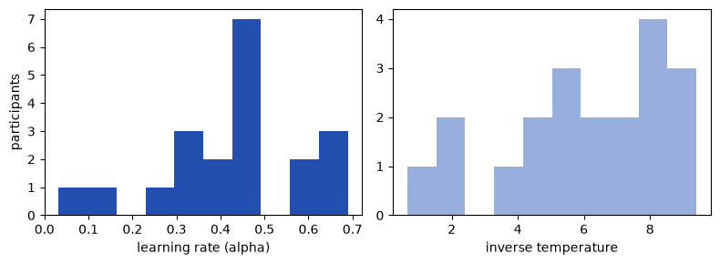
It has two free parameters: the learning rate alpha and the inverse temperature temperature.
A model in cpm is a Wrapper: it runs the computations of one trial over all trials of one participant.
We build it with the data of a single participant; the optimiser swaps in the data of each participant when fitting.
parameters_settings gives the starting value, lower bound and upper bound of each parameter.
Fit it to every participant#
FminBound finds the parameters that maximise the likelihood of the choices of each participant, within the bounds of each parameter.
prior=True adds the priors of the parameters, so the estimates are maximum a posteriori.
from cpm.optimisation import FminBound, minimise

fit = FminBound(
    model=model,
    data=data.groupby("ppt"),
    minimisation=minimise.LogLikelihood.bernoulli,
    prior=True,
    number_of_starts=3,
    ppt_identifier="ppt",
    parallel=False,
    display=False,
    approx_grad=True,
)
fit.optimise()
import pandas as pd

estimates = pd.DataFrame(fit.parameters)
estimates.describe()
| alpha | temperature | |
|---|---|---|
| count | 20.000000 | 20.000000 |
| mean | 0.429274 | 6.072600 |
| std | 0.169301 | 2.441618 |
| min | 0.032525 | 0.658943 |
| 25% | 0.354631 | 4.917123 |
| 50% | 0.452680 | 6.285428 |
| 75% | 0.510143 | 7.971128 |
| max | 0.689269 | 9.404572 |
fig, axes = plt.subplots(1, 2, figsize=(8, 3))
axes[0].hist(estimates.alpha, bins=10, color="#2350b0")
axes[0].set_xlabel("learning rate (alpha)")
axes[1].hist(estimates.temperature, bins=10, color="#98aedd")
axes[1].set_xlabel("inverse temperature")
axes[0].set_ylabel("participants")
plt.tight_layout()
plt.show()
Run the model with the fitted parameters#
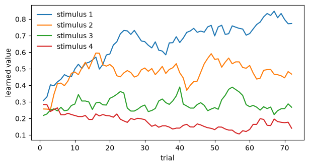
The Simulator runs the model over the trials of every participant, each with their own fitted parameters.
Its output contains everything the model returns on each trial, such as the choice probabilities (policy_0, policy_1) and the learned values of the four stimuli (values_0 to values_3).
| policy_0 | policy_1 | reward | values_0 | values_1 | values_2 | values_3 | change_0 | change_1 | change_2 | change_3 | dependent | ppt | |
|---|---|---|---|---|---|---|---|---|---|---|---|---|---|
| 0 | 0.500000 | 0.500000 | 1.0 | 0.514486 | 0.250000 | 0.250000 | 0.25 | 0.264486 | 0.000000 | 0.000000 | 0.0 | 0.500000 | 1 |
| 1 | 0.500000 | 0.500000 | 1.0 | 0.514486 | 0.250000 | 0.514486 | 0.25 | 0.000000 | 0.000000 | 0.264486 | 0.0 | 0.500000 | 1 |
| 2 | 0.500000 | 0.500000 | 1.0 | 0.685701 | 0.250000 | 0.514486 | 0.25 | 0.171215 | 0.000000 | 0.000000 | 0.0 | 0.500000 | 1 |
| 3 | 0.829271 | 0.170729 | 0.0 | 0.443890 | 0.250000 | 0.514486 | 0.25 | -0.241811 | -0.000000 | -0.000000 | -0.0 | 0.170729 | 1 |
| 4 | 0.500000 | 0.500000 | 1.0 | 0.443890 | 0.514486 | 0.514486 | 0.25 | 0.000000 | 0.264486 | 0.000000 | 0.0 | 0.500000 | 1 |
simulation["trial"] = simulation.groupby("ppt").cumcount() + 1
learned = simulation.groupby("trial")[["values_0", "values_1", "values_2", "values_3"]].mean()

fig, ax = plt.subplots(figsize=(7, 3.5))
for i, column in enumerate(learned):
    ax.plot(learned.index, learned[column], label=f"stimulus {i + 1}")
ax.set_xlabel("trial")
ax.set_ylabel("learned value")
ax.legend(frameon=False)
plt.show()
Summary and next steps#
In a few lines, you fitted a reinforcement learning model to 20 participants and looked at what the model learned about each stimulus.
To build a model of your own from cpm components, work through Tutorial 1: Build and fit your first model.
To check whether estimates like these can be trusted, see Tutorial 2: Parameter recovery.
To see how data, parameters and models fit together, read the core concepts.