Faster fitting in cpm 0.26

28 September 2026 · cpm 0.26.0

The built-in models of cpm now compute all trials of a participant in one call instead of one call per trial, and, when numba is installed, that loop over trials is compiled. Fitting them is 90 to 220 times faster than in cpm 0.25, and more than 1,000 times faster for PTSM2025, with the same results. Your code does not change.

What changes for you

• Install numba with cpm: pip install "cpm-toolbox[numba]". That is all it takes. RLRW, HybridMBMF, PTSM, PTSM1992 and PTSM2025 keep their arguments, parameters, priors and outputs, and give the same results.

• Without numba, the same models run as plain Python, 11 to 23 times faster than in cpm 0.25 (about 250 times for PTSM2025). numba is optional because it supports a new NumPy release only some time after it comes out, and does not support PyPy.

• Your own models are faster too. Every per-trial Wrapper model runs about twice as fast, and you can compile your own models with the new SessionWrapper: see Speed up fitting with numba.

• Hierarchical results change. EmpiricalBayes and VariationalBayes used to discard the population priors they estimated after the first evaluation of each fit. They now use them throughout, so their results differ from cpm 0.25 (see below).

How much faster

Fitting a model evaluates its objective function (the negative log posterior) at one parameter set after another, thousands of times per participant. The figure shows how long one evaluation takes for each built-in model, fitted to one participant.

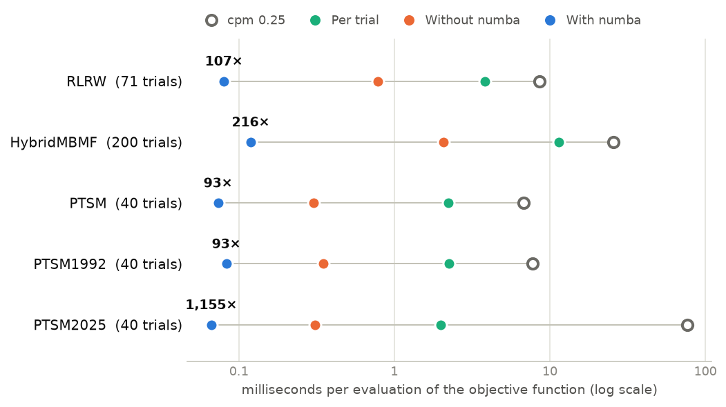
Per trial is a model’s own per-trial function, model(parameters, trial), in a plain Wrapper, which is how you extend a built-in model trial by trial; it runs without numba. Without numba and With numba are the built-in model computing all trials at once.

	Trials	cpm 0.25, ms	Per trial, ms	Without numba, ms	With numba, ms	Speed-up with numba
RLRW	71	8.59	3.83	0.783	0.0802	107×
HybridMBMF	200	25.7	11.4	2.07	0.119	216×
PTSM	40	6.81	2.22	0.301	0.0735	93×
PTSM1992	40	7.72	2.26	0.349	0.0831	93×
PTSM2025	40	76.8	1.98	0.31	0.0665	1,155×

With numba, running the model now takes about as long as computing the loss, and resetting the parameters and evaluating the priors, which took about 1 ms per evaluation in cpm 0.25, take a few microseconds.

Hierarchical estimation

The two hierarchical tutorials, 4. Hierarchical estimation I: empirical Bayes and 5. Hierarchical estimation II: variational Bayes, simulate 50 participants and fit them with two starts each, in 2 chains of up to 6 iterations; each iteration refits all 50 participants. Their model is written out per trial, and is the built-in RLRW model, which gives the same estimates.

In cpm 0.25, the fitters stopped after fewer iterations, because discarding the updated priors made each iteration refit almost the same model. The figure therefore compares the same amount of work: the separate maximum-likelihood fits, and one iteration of each method.

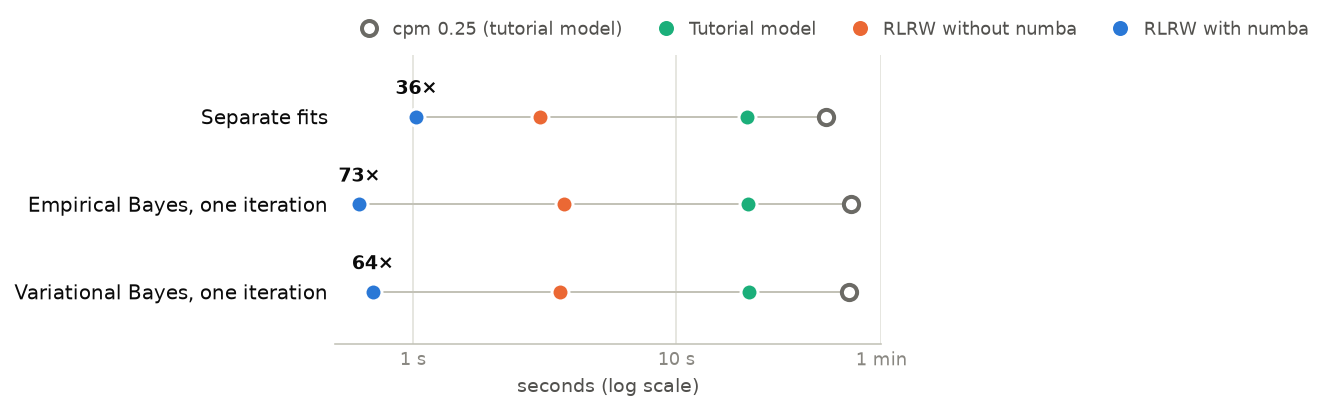
The whole analyses, fitting only, with the number of iterations they ran:

	cpm 0.25, tutorial model	Tutorial model	RLRW without numba	RLRW with numba
Empirical Bayes	496 s (10)	244 s (12)	48 s (12)	8.6 s (12)
Variational Bayes	181 s (4)	228 s (12)	44 s (12)	8.5 s (12)

The tutorials themselves keep their per-trial model, which shows how a model is built from cpm’s components; they run about twice as fast as before.

Same results, and one fix

• The objective function of the built-in models is the same as in cpm 0.25, and so are all their outputs: exports, dependent variables, states and seeded simulations, with and without numba. They are bit-identical on the machine below; on other machines they can differ in the last digit, where numba and NumPy compute exponentials slightly differently.

• The classes in cpm.models give bit-identical results, and the quickstart, the first tutorial and the two-step example reproduce their stored outputs.

• Hierarchical estimation changes, as intended. The table compares the group estimates of the first chain with the group distribution the data were simulated from.

	α mean	α SD	β mean	β SD
True group distribution	0.60	0.20	2.00	1.00
Empirical Bayes, cpm 0.25	0.55	0.30	2.69	2.37
Empirical Bayes, cpm 0.26	0.57	0.20	2.16	0.92
Variational Bayes, cpm 0.25	0.54	0.30	2.63	2.38
Variational Bayes, cpm 0.26	0.55	0.23	2.13	0.98

In cpm 0.25, every participant was fitted with the broad starting priors, so the estimated spread of the inverse temperature β was more than twice its true value.

How we measured

• Machine: Intel Xeon w5-2455X (12 cores), 32 GB, Windows 11; Python 3.12.4, NumPy 2.5.3, SciPy 1.18.1, pandas 3.0.6, numba 0.67.0.

• Code: cpm 0.25 is main at commit 32629af; cpm 0.26 is the development version at commit 830d479.

• One evaluation: python benchmarks/run.py --repeats 300, the median of 300 calls after one warm-up call.

• Hierarchical: python benchmarks/hierarchical.py eb|vb tutorial|rlrw OUT, single runs.

All runs used one thread for NumPy’s linear algebra, ran one at a time, and loaded numba’s compiled code from its cache. The first run of a model with numba compiles it once, which takes a few seconds (up to about 15 s for the prospect-theory models); after that, cpm loads the compiled code from disk. The results on other machines, operating systems and Python versions will differ, but the ratios should be similar. The data behind the figures are in benchmarks/results/ in the cpm repository.

For every change in this version, see the changelog.